Communications Primer

Let's rock and roll. To start off with the most basic definition of [electrical] communication, we're trying to send some message from point A to point B. We do that by encoding whatever message we're sending to binary (just 1's and 0's). These bits, or symbols, don't mean a whole lot in the real world, so we're going to send two signals: HIGH and LOW. If I'm the one sending the bits, I'll the transmitter (TX), and if I'm getting the bits, I'm the receiver (RX).

In normal electronics, we would send $V_{DD}$ and $GND$, but that makes the math slightly annoying. Instead, we'll use differential signals that we'll arbitrarily call $+1$ and $-1$. It doesn't necessarily mean exactly $\pm 1V$, just HIGH and LOW.

Now for some probability! If all of this were purely digital, then we would have a very simple distribution. In this digital domain, we would use a probability mass function (PMF) to describe this distribution. The only rules we need to know are:

1. The probability that any bit is sent is 1

• Every time we send a bit, we also receive one
• P(+1) + P(-1) = 1
• But not necessarily the same one…

2. The odds of sending any bit is independent and identical

• P(+1) = P(-1)

Therefore all we have is a 0.5 chance of getting either bit. Probably intuitive for most, but defining it is always helpful. If we plot this, we get the following graph:

We interpret this by plotting the probabilities of the transmitted bits, and then drawing a vertical line at $X=0$. If we're greater than zero, we can interpret that as a +1, and if we're less than zero, we can interpret that as a -1. Since this is a very simple example, every bit we send is the same bit we'll receive.

Now we can move on to more continuous bits. Instead of doing PMFs, here we look at probability density functions (PDFs) and see what happens. We can obey fairly similar rules:

1. The probability that any bit is sent is 1

• Rather than summing our discrete possibilities, we integrate our continuous ones!
• $P(0.1 < X < 0.3) = \displaystyle \int_{0.1}^{0.3} P(X) \text{dx}$
• $\displaystyle \int P(+1) \text{dx} + \int P(-1) \text{dx} = 1$

2. The odds of sending any bit is independent and identical

• $\displaystyle \int P(+1) \text{dx} = \int P(-1) \text{dx}$

While our transmitted PDF can take a variety of functions, we can start by using simple Gaussian distributions (also known as “bell curves” or “normal distributions”). Here's a simple one plotted below:

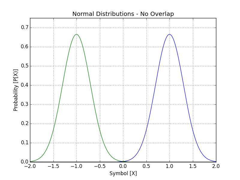
Like before, we still plot the distributions and interpret it around the zero line. If we're higher than zero, it's received as a +1 (blue), and less than is received as a -1 (green). This one (as the title infers) is a non-overlapping set of distributions, so we have no errors in this either. What has changed, however, is how we measure it. In the quasi-digital set, we only needed to check +/-1 exactly, but now, we need to measure from 0 to 2 for +1, and -2 to 0 for a -1. This makes the next stage harder, since we need to have a better “interpreter” - a digitizing circuit that takes the wide-range voltages that get sent and converts them back into bits.

Now let's look at one last case that models what happens in reality. Here, we have a slightly worse transmitter, but it has disastrous consequences!

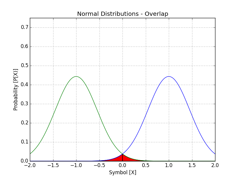
Keeping the same color scheme as before, with blue corresponding to +1, and green to -1 transmitted, things have changed slightly. Now if draw the line at zero, if I send a +1, I could get a +1 or -1, each with some distinct probability. Obviously, most of the time, we'll get the bit that was intended, but not always. This brings up the notion of bit error rate (BER), which tells us how many bits we get wrong in a given transmission. There's many ways to calculate BER depending on how the data is available, here's some of them:

• $\mathrm{BER} = \dfrac{P_{X=+1}(-1) + P_{X=-1}(+1)}{2}$
• $\mathrm{BER} = \dfrac{\text{Number of incorrect bits}}{\text{Total sent bits}}$

So for the above example, we can calculate the BER by using statistical functions. The average error is now:

$$ \dfrac{P_{TX=+1}(X<0) + P_{TX=-1}(X>0)}{2} \approx 2.1% $$

While that seems pretty good, it's absolutely awful for the real world. Most modern clocking circuits need to have a BER on the order of $10^{-10}$ to $10^{-14}$. If we're at 98%, that means 1/50 words were wrong in this post. While I'd actually be pretty happy with that (I'm pretty bad with typos), a computer processor would just completely break down. For reference, in a 1080p monitor, that corresponds to over 40,000 incorrect pixels!