Comb Filter

Back to circuit posting! Right now I'm working through Jake Baker's book¹ and I'd like to do some more simulations myself to get a better handle on it. Let's start with something simple, the comb filter. The motivation here is that we want to remove multiples of some frequency completely, like a notch filter for a certain frequency and it's harmonics. It's a simple circuit to build, all we do is take some input, delay it in time, then add it back to the original input and see what we get. I'll go through this in an analog (LTSpice) and digital manner (SciPy).

Math

Let's start with what we expect to see, then check if that actually happens in a simulator. Mathematically, we have our input signal Vin and we delay it by td, then sum it back to create Vout.

$$\rm V_{out} = V_{in}(t) + V_{in}(t-t_d)$$

Or if we write that in the phase-form rather than time-form:

$$\rm V_{out} = V_{in} + V_{in} e^{-jwtd}$$

Here I'm just curious about the AC performance, or the gain:

$$\rm A_V = \left| \dfrac{V_{out}}{V_{in}} \right| = \left| 1+e^{-jwt_d} \right|$$

We can expand this using Euler's identity for \(e^{jx} = \cos(x) +j\sin(x)\).

$$\rm |1+e^{-jwt_d}| = |1 + \cos(-wt_d) + j\sin(-wt_d)| = \sqrt{\left(1 + \cos(-wt_d)\right)^2 + \left( \sin(-wt_d) \right)^2 }=$$ $$\rm \sqrt{1 + 2\cos(-wt_d) + \cos^2(-wt_d) + \sin^2(-wt_d)}$$

Playing some trigonometric tricks (\(\cos^2(x)+\sin^2(x)=1\) and \(1+\cos(x) = 2\cos^2(x/2)\)):

$$\rm A_V = \sqrt{2 + 2\cos(-wt_d)} = \sqrt{4\cos^2(-wt_d)/2} = 2\left|cos(wt_d/2)\right|$$

Let's check that output with a quick plot:

import numpy as np
import matplotlib as mpl
import matplotlib.pyplot as plt

mpl.style.use('research')
plt.close()

td = 1E-6

f = np.linspace(0, 5E6, 200)
w = 2*np.pi*f

gain = 2*np.abs(np.cos(w*td/2))

plt.xlabel('Frequency [MHz]')
plt.ylabel('Gain [V/V]')
plt.title('Comb Filter Magnitude Response (td=1us)')
plt.plot(f/1e6, gain)
plt.tight_layout()

Now we can see where the “comb” name comes from - all the little ridges ducking in and out just like a comb! The notches start at \(2/t_d\), and repeat every \(1/t_d\).

Analog

Now we need to figure out how to finally build it. For the analog implementaiton, we'll use a simple transmission line to implement the delay. While a 1\(\mu\)s delay might be large, we'll work with it for now. To add the voltages, we can simply tie the two inputs together using resistors. The only difference is that instead of directly using the sum of the two inputs, we'll now use the average of them. This just removes the factor of 2 from our equation, and means our new maximum value is 1. This makes sense, as there's no way to get gain larger than 1 for passive components.

The only trick here is that we need to make sure the transmission line doesn't create any bounces back and forth. To avoid that, we'll terminate the line with a \(50\Omega\) resistor to match the characteristic impedance, then use larger resistors for the summing. Our schematic looks like:

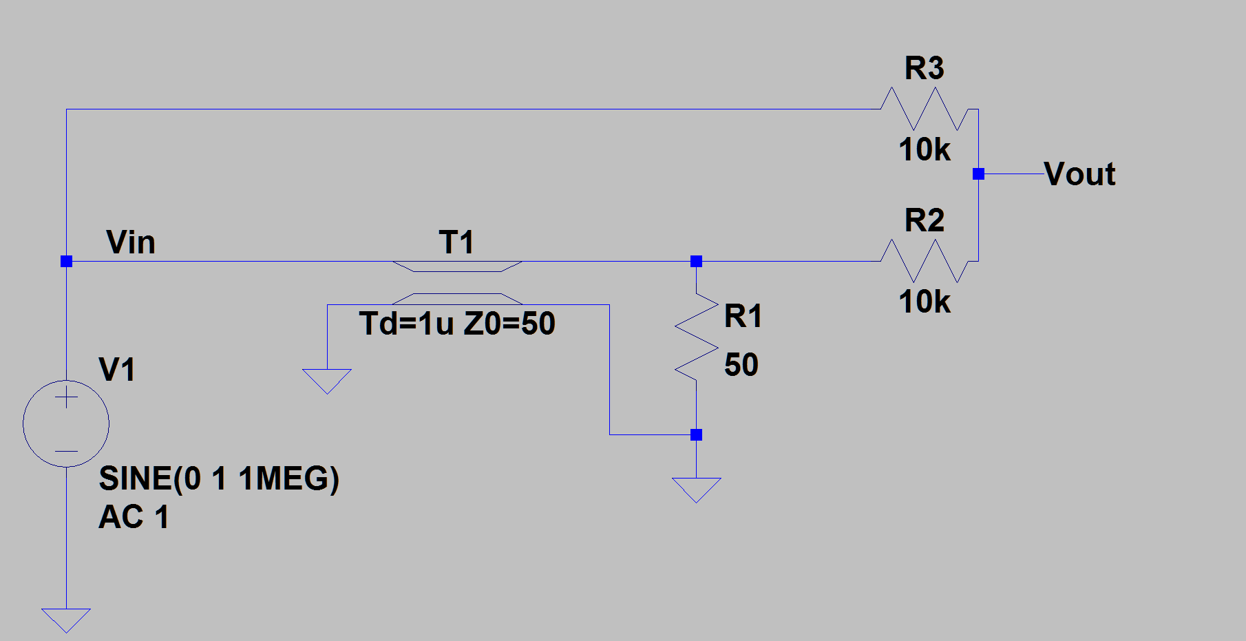
With netlist:

* Comb Filter
* Notches at every Td starting at Td/2
T1 Vin 0 N001 0 Td=1u Z0=50
V1 Vin 0 SINE(0 1 1MEG) AC 1
R1 N001 0 50
R2 Vout N001 10k
R3 Vout Vin 10k
.ac lin 200 10k 10MEG
.end

LTSpice is nice, but I hate it for presenting data. The plotting tool “works” and that's about all I can say. I exported the data and then plotted it again in matplotlib:

import pandas as pd

df = pd.read_table(r'C:\Users\brady\OneDrive\Documents\LTspiceXVII\comb-filter.txt',
                   sep='\t|,', skiprows=1, names=['freq', 'real', 'imag'])

df['mag'] = np.abs(df.real + 1j * df.imag)

plt.xlabel('Frequency [MHz]')
plt.ylabel('Gain [V/V]')
plt.title('Comb Filter using TL')
plt.plot(f/1e6, df['mag'])
plt.tight_layout()

Drumroll please…

Great! If we account for that division by two, it lines up perfectly.

Digital

Last but not least, we should prove it works in a digital system too. A digital delay is just a register block. If we want more delays, we cascade more registers. A longer delay will in turn give us more notches, each linearly spaced between 0 and \(f_s\). Mathematically, I'm simulating:

$$\rm V_{out}[n] = V_{in}[n] + V_{in}[n-k]$$

Or in z-domain:

$$\rm A_V = 1 + z^{-k}$$

I'll simulate it in Python:

from scipy import signal

#weights = [1, 1]
weights = [1,0,0,0,1]
w, h = signal.freqz(weights, whole=True)

plt.plot(w/(2*np.pi), 20*np.log10(np.abs(h)))

plt.xlabel('Normalized Frequency ')
plt.ylabel('Magnitude [dB]')
plt.ylim([-30, 10])
plt.title('Digital Comb Filter ({} tap delay)'.format(len(weights)-1))
plt.tight_layout()

Which gives us the following outputs:

Great! Same as before. I think that's enough about comb filters for awhile.